Forward Kinematics Transform
Purpose in the Pipeline
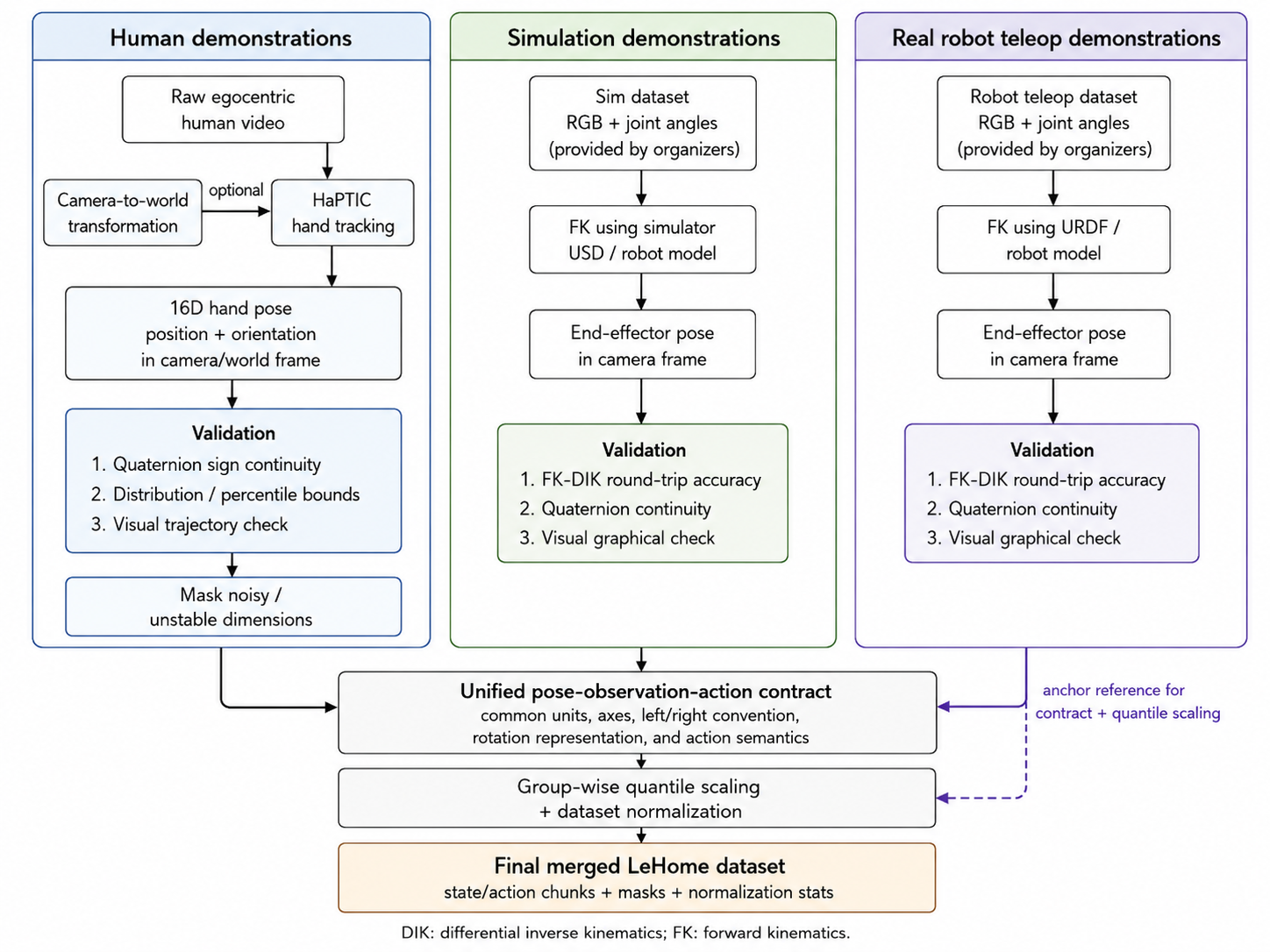
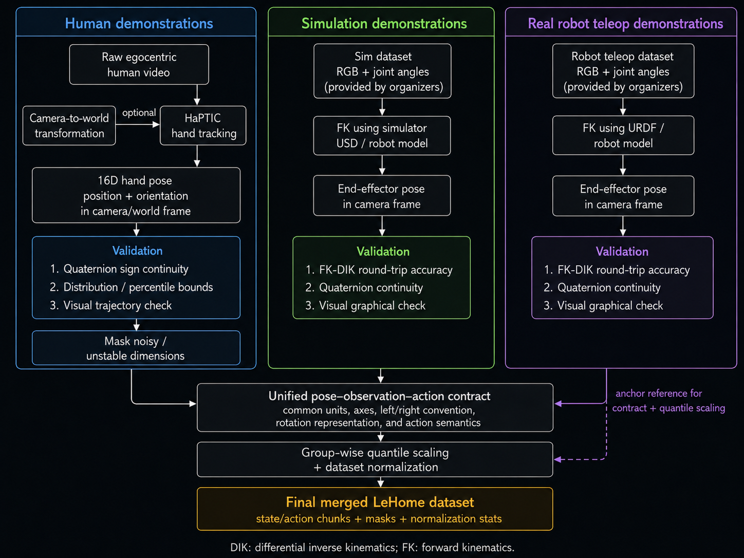
The forward kinematics transform is the component that makes robot data comparable with the
human demonstration data. The LeHome simulation and real-robot teleoperation logs are provided in the
native robot joint representation: six values for the left arm and six values for the right arm. Human
demonstrations, however, do not have robot joint angles. They are closer to a pair of hand or
end-effector trajectories observed from the camera.
Instead of trying to retarget human motion into robot joint angles, the pipeline converts the robot data
into the same representation family as the human data: a dual-arm end-effector pose. This is why forward
kinematics is applied to the organizer-provided simulation and real-robot teleoperation datasets. It turns each
12D joint state or action into a physically meaningful 16D pose in the camera frame.
Input and Output Representation
For each frame, the native robot state is represented as a 12D vector. The first six values correspond to
the left arm, and the next six values correspond to the right arm. Each arm contains the shoulder, elbow,
wrist, and gripper values used by the LeHome robot.
\[
\mathbf{q}^{12} =
\left[
\mathbf{q}^{6}_{L},
\mathbf{q}^{6}_{R}
\right]
\]
\[
\mathbf{q}_{L}^{6} =
\left[
q^{L}_{\mathrm{shoulder\_pan}},
q^{L}_{\mathrm{shoulder\_lift}},
q^{L}_{\mathrm{elbow\_flex}},
q^{L}_{\mathrm{wrist\_flex}},
q^{L}_{\mathrm{wrist\_roll}},
g_L
\right]
\]
The arm joints are used to compute the end-effector transform. The gripper value is not part of the
spatial rigid-body transform, so it is copied into the final per-arm pose. Each arm is represented as an
8D pose: three position values, four quaternion orientation values, and one gripper value. Concatenating
the left and right arm poses gives the final 16D pose.
\[
\mathbf{p}^{8} =
\left[
x,\ y,\ z,\ q_w,\ q_x,\ q_y,\ q_z,\ g
\right],
\qquad
\mathbf{p}^{16}_{C} =
\left[
\mathbf{p}^{8}_{C,L},
\mathbf{p}^{8}_{C,R}
\right]
\]
How the Kinematic Chain Is Evaluated
Forward kinematics starts at the robot base and walks through the kinematic chain one joint at a time.
Every joint contributes a fixed transform from the parent link into the joint frame, a motion transform
determined by the current joint value, and a fixed transform from the joint frame into the child link.
Multiplying these transforms in sequence gives the end-effector transform.
\[
T = T^{W}_{B}
\]
\[
T \leftarrow
T
\cdot
T_{\mathrm{parent},i}
\cdot
T_{\mathrm{motion}}(q_i)
\cdot
T_{\mathrm{child},i}
\]
For a revolute joint, the motion transform is a rotation around the joint axis. For a prismatic joint, it
is a translation along the joint axis. The LeHome arm primarily uses the actuated serial chain to recover
the wrist or end-effector transform, while the gripper value is carried as a separate scalar.
\[
T_{\mathrm{motion}}(q_i) =
\mathrm{Rot}(\mathbf{a}_i, q_i)
\quad \text{or} \quad
T_{\mathrm{motion}}(q_i) =
\mathrm{Trans}(\mathbf{a}_i q_i)
\]
World Pose to Camera Pose
Once the chain is evaluated, the result is the world-frame end-effector transform. The translation part
gives the end-effector position, and the rotation matrix is converted into the quaternion convention used
by the policy.
\[
T^{W}_{ee} = \mathrm{FK}(\mathbf{q}),
\qquad
\mathbf{x}^{W}_{ee} = T^{W}_{ee}[0:3,3],
\qquad
R^{W}_{ee} = T^{W}_{ee}[0:3,0:3]
\]
The policy uses camera-frame poses rather than raw world-frame poses. Therefore the world-frame
end-effector transform is mapped into the calibrated camera frame using the camera extrinsics. This
produces the final 16D camera-frame pose that is used as the model state and action target.
\[
T^{C}_{ee} =
T^{C}_{W} T^{W}_{ee}
\]
\[
\mathbf{p}^{8}_{C} =
\left[
x^{C},\ y^{C},\ z^{C},\ q_w^{C},\ q_x^{C},\ q_y^{C},\ q_z^{C},\ g
\right]
\]
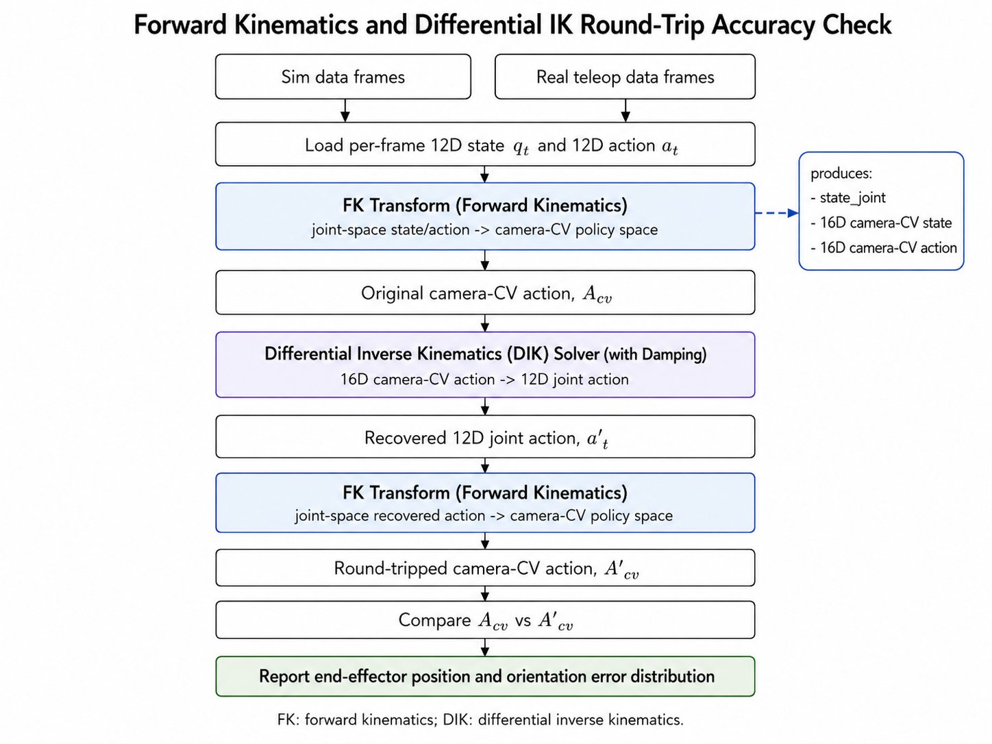
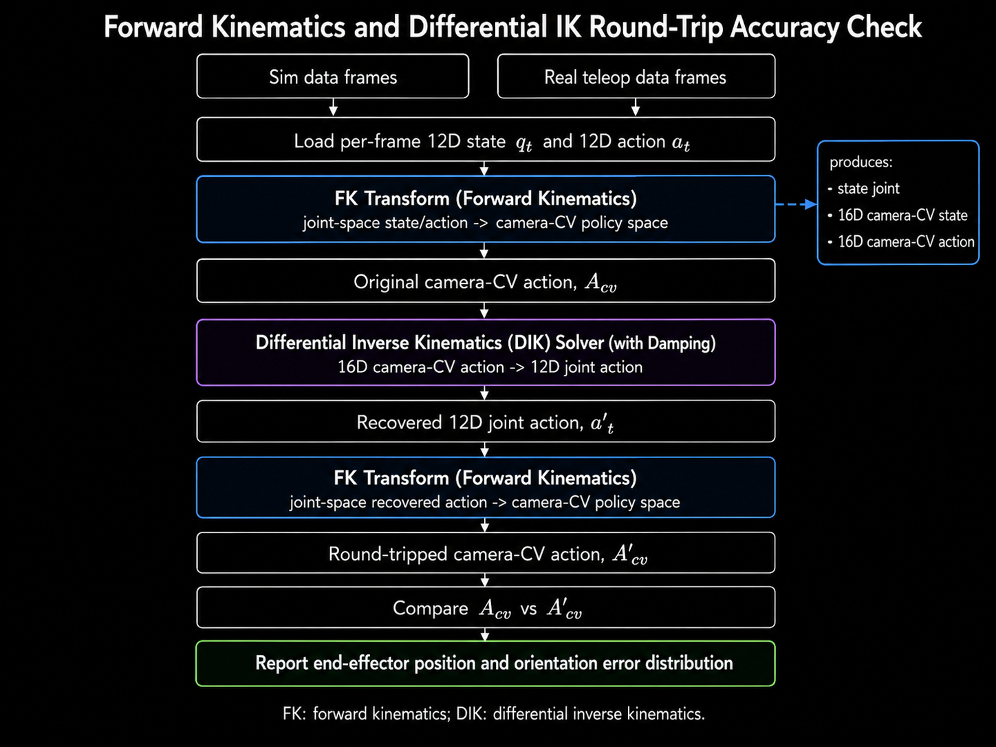
Why the Jacobian Is Computed in the Same Pass
The same kinematic traversal is also used to compute the spatial Jacobian. The Jacobian describes how a
small joint change affects the end-effector position and orientation. This is not only useful for
analysis; it is required by the differential inverse kinematics solver used during deployment.
For each actuated joint, the implementation stores the joint axis in world coordinates, the joint origin
in world coordinates, and the current end-effector position. For revolute joints, the linear component is
the cross product between the joint axis and the vector from joint origin to end-effector. The angular
component is simply the joint axis.
\[
\mathbf{J}_{v,i} =
\mathbf{z}_i \times
(\mathbf{p}_{ee} - \mathbf{o}_i),
\qquad
\mathbf{J}_{\omega,i} =
\mathbf{z}_i
\]
\[
J(\mathbf{q}) =
\begin{bmatrix}
J_v \\
J_{\omega}
\end{bmatrix}
\in
\mathbb{R}^{6 \times N}
\]
Role During Training
During training, forward kinematics is applied to the simulation and real-robot datasets so their native
12D joint states and actions become 16D end-effector pose states and actions. The human demonstrations
are already closer to this pose format after hand-pose processing, so the FK conversion lets all three
sources meet in the same policy-facing representation.
\[
\text{simulation robot joint data}
\xrightarrow{\mathrm{FK}}
\mathbf{p}^{16}_{C},
\qquad
\text{real-robot joint data}
\xrightarrow{\mathrm{FK}}
\mathbf{p}^{16}_{C}
\]
\[
\mathbf{a}^{12}_{t}
\xrightarrow{\mathrm{FK}}
\mathbf{a}^{16}_{C,t}
\]
This avoids mixing human pose data with robot joint-angle data directly. Instead, the policy sees one
consistent camera-frame pose-observation-action contract across human, simulation, and real-robot data.